Process variables and the art of calibrating instruments

Jim McCarty is systems developer in Minneapolis for Optimation, a system integrator headquartered in Rush, New York. He is a certified LabView developer and certified professional National Instruments instructor. McCarty has more than eight years of experience in application areas such as the medical device, solar, semiconductor, defense, transportation and mining industries. Contact him at [email protected].

Let’s start with the basics of calibration: the output of an instrument is measured under one or more known conditions (for example, the current output of a pressure transducer may be measured at 0 and 100 psig), and then a function of the sensor output (typically a linear function, so just a slope and an intercept) is generated to calculate the measured value of the sensor anywhere in that measurement range by knowing the output of the sensor.

Theoretically, in the example of a pressure transducer, this means that you can throw a digital multimeter (DMM) on a transducer and measure it sitting in the open, connect it to a shop air line, measure it with the DMM again, and be done after the calculation of the slope and intercept of the line that you draw through the points on a pressure vs. output current plot. However, there are critical points for not only performing a good calibration, but also making sure that it remains good:

• The stimulus (input—pressure, temperature, flow) is very accurately known.
• The calibration procedure yields repeatable and reproducible results.
• The stimuli/conditions are stable.
• The conditions represent the entire test range (if you expect to measure 0-100 psig on your test system, then you should calibrate at or near 0 and 100 psig) and test the sensor linearity.
• The calibration is performed under the same conditions as the measurement is made using the test system.
• The analysis is performed correctly, with passing and failing criteria.

Let’s step through each of these and discuss how they are relevant to a cleaning skid, so that we can build an effective and efficient calibration procedure. I’ll spend the most time on the first two topics, as they are arguably the most important, as well as a good chunk of time on the last topic, as I feel that it’s often overlooked. I’ll be using flow meters, pressure transducers, and thermocouples as examples.

Before diving into the details, first determine what your measurement accuracy must be, as calibration accuracy has a huge influence on measurement accuracy.

The stimulus (input) is very accurately known

Accurately knowing what you’re measuring is possibly the single most important point when it comes to calibration because the instrument being calibrated will carry whatever this error is (difference between what you think you’re measuring during calibration and what you’re really measuring) into the test system. Simply stated, if you think you’re measuring 100 psig in calibration, but the pressure is really 98 psig, you’ll report 98 psig whenever the pressure in your system is actually 100 psig, even if you’ve done everything else perfect.

I will also mention here that, in your analysis, you should always use the exact measured stimulus and sensor output values in your calibration calculations and analysis. The way I see this not implemented is when the procedure calls for nominal data points every so many psig, sccm or degrees at some sensor output current. It’s only important that you hit these points very approximately, but if you’re going through the trouble of measuring exact quantities, use the exacted measured quantities, not some nominal value a procedure calls for.

This typically stipulates that a known, accurate reference instrument (often informally called a “golden unit”) must be used in the calibration setup to be measured alongside the sensor you’re calibrating, or the device under calibration (DUC), or at least be used somewhere in your overall calibration process. Some sensors can be calibrated at some values without one—for example, static torque can be applied using a fixture arm and a weight and then measured by a torque cell, and there are some “stakes in the ground,” such as the density of water—however, in many industries, these gems are few and far between. These are also how primary standards are generated.

Golden units are typically only used for calibration in order to minimize usage and therefore decrease the probability of breaking them, and furthermore are stored in a safe place when not in use. As you can probably imagine, a faulty golden unit can cause quite a stir, as it serves as your “sanity check,” and for this reason many labs calibrate reference sensors (think of them as clones of your golden unit) off of a single golden unit. Typically, these references are used when either running a test that requires a reference instrument or to calibrate test systems, and the golden unit is only used to calibrate the references monthly, or less frequently.

You may hear the terms “primary,” “secondary” and “working” standard. A primary standard is a sensor that is calibrated against some known stimulus, boiling down to manipulating quantities like mass, time and length, if possible, instead of another sensor—so instead of minimizing calibration error due to the stimulus being unknown, this error is removed entirely. Secondary and working standards are sometimes, but rarely, used interchangeably in the context of calibration standards, but the secondary standard usually implies a much closer approximation or much more similarity to some primary standard, as more care is taken to keep them in consistently the same working condition, often implying far less usage than a working standard.

Having a single golden unit is common because it’s usually either costly, time-consuming or both to maintain a sensor’s golden status. “Golden” may also imply that it’s a primary standard, but not always. A typical process may be to send it to the manufacturer or other third-party calibration lab annually (the costs are typically paid by you if they do this, and it’s often not cheap), with the device being gone for about six weeks. Whenever the golden unit is recalibrated, the references should be recalibrated against it. The best way to do this, to avoid tolerance stacking, is to calibrate all references against the golden unit in the same calibration run, compared to calibrating Reference A against the golden unit, then calibrating Reference B against Reference A, then Reference C against Reference B, D against C, and so on. In the latter case, the error accumulates run to run.

A golden sensor doesn’t necessarily have to be a more accurate or precise model compared to the sensors it is used to calibrate, but you need to be assured, somehow, that its reading is accurate (so, at the same time, more accurate and precise doesn’t hurt). If the sensors you are calibrating are known to be not so great when it comes to accuracy or precision, then you probably need a nicer-model sensor for the golden unit. It may be worth it, for example, if your pressure-measurement accuracy requirement is tight and your boss’ or customer’s pockets are deep enough, to shell out for a few very nice pressure gauges or transducers.

I swear by Ashcroft for gauges and Druck for transducers, if you’re able to find them, as they’re not commercially available in the United States anymore.

So, armed with a golden reference sensor, how do you induce some meaningful condition for calibration?

Establishing some stimuli, such as pressure, is relatively easy—simply measure the DUC on a vessel with a vent or other outlet open, or with the transducer off of the vessel at ambient pressure, then attach the DUC and golden transducer, pressurize the vessel, wait for stabilization and measure. To get your in-between points, use a pressure regulator or pump attached to the vessel.

Establishing some stimuli, such as a stable, accurately known flow, can be difficult. However, establishing a known volume or mass and a known period of time is significantly easier. By definition, flow is how much mass or volume is passed in how much time, so most flow meters are calibrated by passing a known volume of fluid through the meter over a known period of time, and then sensitivity is calculated, assuming volume, as:

Think simple, like pouring water from a beaker or bucket into a funnel and through a flow meter, or into a system with a flow meter. If your fluid is a gas, you can use a similar approach with a known volume or mass over time, but the implementation isn’t as simple, of course. Using this method, maintain a steady flow over the course of the measurement period, and use a high sampling rate, if possible. Both will minimize the effect of transients—spikes and dips in the real flow—not being measured.

With flow meters, it’s important to use the same or similar fluid that will be measured in the test system, as viscosity, density and temperature will all affect a flow measurement. This may be a matter of starting the data acquisition at, say, 20 Hz, and then pouring exactly 1 gal of water into a funnel and through the meter and then terminating the acquisition. When you’re using a 4-20 mA output sensor, this implies that there’s some non-zero nominal offset at zero flow, so you should also perform a null measurement, in which you measure the output of the flow meter with zero flow for some period of time and then take the average, which is the term in the equation above.

Some conditions, like temperature, can be very difficult to induce at all, depending on the setup, let alone inducing them in a known way. Luckily, for temperature calibration, we don’t care so much that we’re hitting exactly some temperature in calibration; we only care to know exactly what we’re hitting in calibration, and, of course, that we’re not melting, vaporizing or letting the smoke out of anything in the process. For some temperature sensors, you only need to correct for some offset in the sensor or the system, and this will be sufficient. This simply means that you measure the DUC output at any single known temperature. Can you get away with this?

Find out—measure the DUC output at some known temperature. To find the temperature, use your golden temperature sensor; if the sensor you’re calibrating is removable, a water bath or a metal plate are both simple and will stabilize your DUC and golden unit to the same temperature, assuming you’re not doing anything funny like heating on end of the bath or plate. If not, you still need to get the golden unit to the same temperature as your DUC somehow, so be creative—thermally conductive paste or putty will most likely be very useful. Now heat or cool both the DUC and golden unit to approximately the upper or lower temperature extreme—again, think simple—hot or cold water, a hot plate or even your thumb or a piece of ice may do, as we’re just trying to get it hot or cold at this point.

Also read: Don't let poor wire and cable decisions slow down your next project

If your DUC isn’t removable, remember that an electric heater is just current flowing through something that has non-zero resistance, so heaters can come in small, simple, portable, convenient packages, such as cartridge heaters. Using the calculated offset from the ambient temperature case before you heated or cooled the DUC, how far off is your hot or cold measurement from your DUC vs. your golden unit? If it’s acceptable, then all you need to do is the first ambient measurement. If not, then you’ll need to repeat what you just did—the ambient and the hot or cold measurement—for routine calibration. Again, the important parts are that the DUC reaches a temperature close to one of the limits (far enough away from ambient) and that the DUC and golden unit are at the same temperature, so it doesn’t have to be pretty, nor does it have to be at the exact same temperature for every calibration you run; of course, it does have to be safe and probably not terribly messy, so don’t get too crazy.

Recap: Have one very accurate golden unit for each sensor type, and clone references whenever it’s recalibrated. When creating these clones, avoid tolerance/error stacking whenever possible. Induce your stimulus in such a way that it’s accurately known. If it’s not possible to induce the stimulus in such a way that it’s induced when the sensor is in normal operation with it being accurately known, be creative and induce it in a way that you might know some other quantity that correlates to the quantity of interest. Above all else, at this point, focus not so much on how you induce a stimulus, but instead how you’ll most accurately know what exactly you’re inducing on your DUC.

The calibration procedure yields repeatable and reproducible results

Let’s quickly recap what “repeatable” and “reproducible” mean.

• If a process is repeatable, that means that you can go back into the same lab with the same part and, using the same test station, get the same results. You can repeat what you did.

• If a process is reproducible, that means that I can follow that same procedure in a different lab and different part (same model though, of course) and, on a presumably different test station, get the same results you did. I can reproduce what you did.

This means that any measures or processes that force us to do the same things in the same ways from calibration to calibration are good.

Software repeatability and reproducibility

Putting the calibration into the software is probably the single best thing you can do for repeatability and reproducibility (R&R). This also helps to enforce good laboratory practices when it comes to data collection, and most software can also force the physical calibration procedure to be executed the same way.

Without calibration being part of your software, most software can be operated just by entering sensitivity and offset values, and you effectively lose any enforcement of traceability, as well. Think about the user just entering values on a user interface or in a text file and saving it. If you suspect that you got bad test results because of a bad calibration, that's all you know, or all you think—your information trail ends there. You have no record of what reference sensor was used (maybe a specific reference is suspected of going bad); what the calibration data looked like (maybe there were outliers in the data that threw off your sensitivity and/or offset); what range it was calibrated over (maybe whoever did it was in a rush and measured at two convenient points at the lower end); or if the sensitivity and/or offset were even calculated correctly (did somebody fat-finger an extra digit in one of the values?). This, of course, assumes that things like DUC serial numbers, reference serial numbers and the raw data itself are all stored in some log file for each calibration.

Of course, the question "but is it worth it?" will come up, with "it" being the effort required to add this into your software or build another application to handle calibration. Personally, as somebody who's writing a lot of software lately, I think this is a no-brainer—the math, the most complicated part being the least squares fit, is relatively straightforward, and any submodules required to at least set up and read your DUCs are most likely already written. Within the medical-device environment, for example, where, in my experience, you need to go through a fairly exhaustive validation process whenever you breathe on previously validated code, the calibration functionality can be pretty well isolated from other parts of the code, so you likely won’t need to re-validate much of the existing code.

Hardware repeatability and reproducibility

Are your DUCs, or DUCs-to-be, removable from the test system? If so, then it is preferable to remove them and place them all in one fixture for calibration; fixtures are key to repeatable calibration measurements. The emphasis of the designs I’ll describe is on the references and DUCs seeing the exact same stimulus—that is, the same pressure or temperature.

For pressure calibrations, a simple, inexpensive and small fixture I’ve used is what I call a transducer tree. It’s made up of several female quick-disconnect (QD) fittings piped together; of course, this assumes that your transducer fittings are male QDs, so use whatever mates with your DUCs. Two fittings are reserved for your reference and regulator, and the rest are for your DUCs, although experience has taught me that it would behoove you to build a ball valve to use as a vent on there, too. It doesn’t matter if you have enough DUCs to fill the slots on the tree, as unconnected female QDs don’t bleed air, unless you’re doing this considerably hotter or colder than room temperature, in which case they may leak as badly as a screen door on a submarine, depending on the brand. Because of the small total volume of the QDs with piping, stabilization wait times are minimized over using a big tank or other reservoir.

For temperature calibrations, think of something, maybe somewhat large, that will have a uniform temperature inside of it or on the surface of it that you can attach all DUCs and the golden unit to, and, if necessary (if you determined from the last section that you need to measure at two temperatures), something that you can make hot or cold enough without its breaking or causing other bad things to happen. Again, the goal is just to get the DUCs to a temperature that is known, so this can be as simple and as unpretty as a metal plate or water bath.

Flow meters typically can’t be removed from a setup too easily if they’re already installed, so putting together a fixture may only be worthwhile if you’re calibrating uninstalled sensors. If this is the case, the connections of the DUCs will drive a lot of the design. Try to use as few adapters as possible, and keep the whole thing straight. Adapters and turns in the piping create disturbances that affect flow measurements, so keep the flow though the entire fixture as laminar/straight/undisturbed as possible. You could use a reference for this and attach it to the fixture, or you could use the same approach from the previous section—known volume over a known period defines the flow, not a reference measurement—and save some money and most likely get better accuracy, too. Another seemingly obvious pitfall to avoid meters on branched paths. Make sure that the flow through each meter is identical.

Are your DUCs permanently mounted in your test system, or would it be a complete pain to get them out? If so,, you’ll need to be creative in delivering the stimulus to the DUCs.

For pressure measurements, can you essentially short all DUCs together so that they’re all at the same pressure? For example, a freight train braking system is designed such that the brake cylinder, starting at some relatively lower pressure or at atmosphere, and the various reservoirs, starting at some high pressure, typically 90 psig, equilibrate when a leak or a rapid decrease is detected in the pneumatic signal line pressure—which is also the system supply, called the brake pipe, and runs the length of the train—by opening various paths between the reservoirs, so that they all end up at around 70 psig.

Is it possible to short all the pressure DUCs together like this? If you can’t get the whole system at one pressure at one time, can you open a series of valves or relays that would allow you to do it in parts, where some valve sequence shorts the reference to DUCs A, B and C, and another sequence shorts the reference to DUCs D, E, and F? This may be your next best option. And is there a place—quick-disconnect or other fitting—on your test system for your reference? If not, you’ll have to either make/attach one or move it to multiple spots during the calibration.

Can you do something similar with the system flow? If each flow meter is positioned such that all fluid flow serially through it and no DUCs are on any parallel/branched paths, you’re in luck. And, if the system also lends itself nicely to having a known volume pass through it in a known period, then take the same approach as outlined in the previous section. Just make sure that fluid in = fluid out. You don’t accumulate fluid you pour in or start with an empty system.

If not, look for any way you can induce a known flow and measure the DUC via some unique system feature—for example, if you can allow fluid at a known pressure go through a choke of a known size. If you’re still out of luck, then your best options may be to bite the bullet and either pull the DUC out of the system or measure the flow with some reference unit next to the DUC. Both will likely involve breaking connections, unlike going with the first option and using an ultrasonic flow sensor, which attaches to the outside of the pipe, but can cost between $2,000 and $10,000. This cost can be pretty easily justified by calculating the cost of labor associated with making and breaking connections, if calibration is done frequently enough.

If a temperature sensor is stuck on a system, then thermal paste or grease is very helpful. Apply some to your reference and you can put it next to the DUC and get an accurate reading. Need to make a second measurement at an elevated temperature? A cartridge heater with a thermocouple on the end of it may do the trick. If your DUC is stuck in some component of the system, then you need to do some head scratching. The reality is that you can’t measure temperature at a point in space that isn’t accessible, so there is no easy way out of validating a method for this one. However, there are close approximations that can be proven with data. For example, if a thermocouple is embedded in a ½-in plate, place reference thermocouples mounted on both sides of the plate and heat one side. How far off are the plate temperatures from each other? If they are within some acceptable tolerance, then you can measure with your reference on the surface of the plate to measure the DUC. From here on out, without getting into thermal modeling of the system, it boils down to trying things like this and seeing what will be a close-enough approximation.

The “brute force” approach to temperature calibration, which I usually equate to extra time and effort, would be to heat up the entire system while it’s idle, perhaps in an environmental chamber, and wait for thermal stabilization before making your elevated measurement. Establishing this wait time requires some investigation, for the sake of repeatability and reproducibility. A good place to start would be taking a test system at ambient temperature, putting it in an environmental chamber and recording the sensor temperatures vs. time. Uncalibrated signals are fine; you’re just looking for the signals to plateau. If your lab is set up for it, to get a worst-case stabilization time, try first stabilizing the test system at some considerably lower temperature and then put it in the hotter environmental chamber and determine the stabilization time. Just be aware of the possibility of thermal shock the hotter and colder you go when you try this. Because accuracy is fairly well guaranteed, all sensors will be at the same temperature simultaneously, and not much, if any, re-wiring or attaching/re-attaching is required; this certainly isn’t a terrible idea, but nonetheless it requires the most time for thermal stabilization, and I highly doubt you’ll find an environmental chamber at the dollar store.

With the proper fixturing and the process being controlled in your software, you’ll be guaranteed good repeatability and reproducibility for your calibrations, which typically means the same for your measurements.

Stable conditions and stimuli

You need to be patient and aware of the nuances that can affect particular measurements. However, there are some important general pointers. It’s a good idea to at least be able to measure the output of a sensor continuously at a relatively high sampling rate for an indefinite amount of time in order to study your system.

Short-term stability: The high sampling rate will give you a good indication of the nature of your measurement noise, and measuring for a long time will yield information on stability. Noise is sometimes well understood (for example, 50/60 Hz common mode), and sometimes not. The key to understanding the nature of the noise unique to your test environment and sensors is to select a high enough sampling rate. If you zoom in on the time axis and autoscale the amplitude axis of just about any idle sensor (measuring a constant value) and the points appear to have no flow, then the sampling rate is probably too low for the goals of this pseudo-study. Increase the sampling rate until the points appear to form a more natural looking line, even if the line appears to go up and down at random. Next, look at the periodicity in the noise, imagining the dips and spikes as half cycles of a sine wave. If you were to take a guess at the minimum and maximum frequencies of these imaginary, superimposed half-sine cycles, what would they be?

Your raw sampling rate should be, at the very least, twice the maximum frequency of the noise, per the Nyquist Theorem. Your reporting sampling rate will be much lower—half of the minimum noise frequency, at most. One reported point will be the average of multiple raw points. This way, you’ll be assured that you’re taking the average across at least one “noise cycle,” and the data that you report won’t be so noisy. If you need to report data as quickly as possible, repeat this for measurements under a variety of conditions to find worst-case noise scenarios. You never know when or how noise will affect your measurement. For example, are there any semiconductor devices in your instruments or that affect your instrument readings? Noise in semiconductor circuits generally goes up with temperature, so repeating this at the upper end of the operating temperature range is normally a good idea.

Long-term stability: Sampling indefinitely will give you an idea as to what kinds of stabilization times are required. Think of slowly varying things that could possibly affect your measurements and experimentally determine how much it actually does. Write down anything you can think of, even if it sounds stupid, that could possibly have an effect on the measurement.

For example, do you need to let your pressure transducers warm up in order for them to be accurate? Find out by electrically connecting to one that isn’t pressurized and waiting about 20 minutes while recording data. Look for any changes in the data—does the noise get better, get worse or stay about the same? Does the transducer output rise or fall and then stabilize at some value? What about if you repeat this with a transducer that’s attached to a pressurized vessel? If you’re using the transducer tree from the previous section and, starting at atmospheric pressure, pressurize the tree to 100 psig and record data the whole time, how long does the current signal take to stabilize? What if you used your system to tie all the transducers together at one pressure instead of the tree? Would you have to wait longer for stabilization because of the increased vessel volume? If you just tried that with a transducer that was off just before you started, try it again—does the behavior change if you’re using a transducer that’s already warmed up? What about doing everything with a flow meter? With a thermocouple?

Ask more questions like this, and then go out and get the answers. Theory can answer some questions that may pop up—for example, the answer to “do you have to wait longer for stabilization because of the increased vessel volume?” is a definite yes because of the laws of compressible flow—and guide you to some factors that are somewhat likely to have an effect. Remember what I said about semiconductors and temperature? Knowing this, wouldn’t you think you should at least look into instrument stabilization time after power-up? This will also weed out things that don’t matter. If you’re wondering whether thermocouple warm-up time has any effect, a little research on the Seebeck effect will show you that the thermocouple itself is never powered. However, if it’s converted to a 4-20 mA signal, the signal conditioners may require some warm-up time.

Stepping through these experiments will determine your instrument warm-up times; identify the stabilization period required at a condition such as pressure, flow or temperature to measure a data point; and also shed light on things that should be avoided during calibration, as well as during the measurement itself.

Test-range conditions and sensor linearity

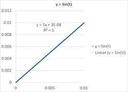
Figure 1: For this range, the data is very well approximated by this linear function, with this specific slope and intercept.

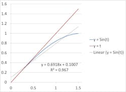
Figure 2: The linear function, fit to only the first portion of the data, shows high error when used to estimate in other parts of the domain, as well as significant disagreement with the linear fit of the entire data set.

A fundamental concept of numerical approximations is that you can make anything linear by zooming in close enough in the time domain. What this means is that you can plot just about anything vs. anything—for example, resistance vs. applied pressure, which is what’s going on at the device level in a pressure transducer—zoom in on a small range on the x-axis, and the points will form what appears to be a straight line. You can also do this with functions that are clearly not linear. If you plot y = Sin(t) for 0 < t < 0.01, it will look like a straight line. You can fit a straight line to this range and come up with an equation (y = x, or the small-angle approximation, assuming you’re working in radians), so we can say Sin(t) ≈ t over this range (Figure 1).

However, expand the higher end of the domain to π/2, and it looks nowhere near linear. Furthermore, if we use the same y = x equation to predict the output of y = Sin(t) in this range, you can see that, once we’re get past ~0.5, our error gets very large. You can go through the motions of fitting a straight line to this new data set (y = 0.692x + 0.101), but you’ll notice your R² value is pretty far off from 1 (0.967), and the line really doesn’t come close to the vast majority data points over the whole range (Figure 2).

To summarize, if we stay within some range, we can use a linear equation to accurately determine the output of the function, but if we wander too far outside of that range, that linear function may yield bad results compared to the actual value. This also highlights the importance of taking multiple points between the minimum and maximum. Would we have had any idea what the curve was doing in between these points? If we had only a couple in between, would this tell us that our linearity is off?

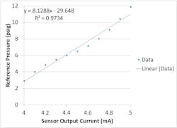
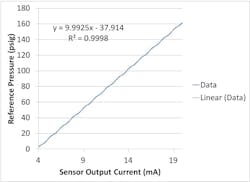
What if we fit a straight line to experimental data from, say, a sensor whose output is known to be linear over some large range, but only use data from a limited range? Look at plots of what the output of a nominal 0-160 psig pressure transducer with a 4-20 mA output might look like, the first only up to ~10 psig and the second covering the whole range (Figures 3 and 4).

In this case, the output of the DUC is linear over the entire range, but, by using only the lower range data, we cut our sensitivity by more than 20% and our offset by ~8 psig. The short and valuable lesson here is that you always want to calibrate over your entire measurement range.

Figure 3: This is a calibration data plot for a range between 0 and ~12 psig, with a calculated sensitivity of 8.13 psig/mA and -29.65 psig offset.

Figure 4: This is a calibration data plot for a range between 0 and 160 psig, with a calculated sensitivity of 9.99 psig/mA and -37.91 psig offset.

In the previous case, though, you could argue that, instead of using a simple linear function, you could fit a quadratic or cubic polynomial or, better yet, interpolate between your data points so that you theoretically have zero calibration error. I would highly advise against this because the majority of sensors are designed so that their output is linear, and, if it isn’t linear, then something is probably very wrong with the sensor. You may be able to try this with a sensor that’s on the edge of going bad and even be able to repeat the calibration a few times and get about the same results for the function coefficients, but there’s a good chance that the sensor will go completely bad soon, and the law of probability says that this will most likely be during a test, not a calibration—you’ll spend a lot more time trying to chase down the issue after you first see the funny results, after it finally goes bad.

Always calibrate over the entire range, and take as many data points as necessary to detect nonlinearities in the sensor output in order to minimize calibration error, as well as detect faulty sensors.

Calibration under test conditions

This ties back into the investigations on what can affect your measurements. You can spend a great deal of time investigating what will have appreciable effects, but I almost guarantee you’ll miss something in the upfront investigation when you’re laying out this process. However, if you do your best to calibrate under the same conditions you’re testing in, the things you do miss are more likely to be undiscovered curiosities, instead of problems you eventually spend a great deal of time trying to track down and fix. Look at it this way: if you’re at this point and you don’t know if and how humidity affects pressure transducers, it’s better not to find out at all because calibration and test happen in the same environment, rather than eventually finding out after being tasked with explaining why you’re calibration process isn’t working. Is your lab actually in a clean room, while the test systems are housed in, more or less, a garage type of environment? If so, it’s probably a bad idea to perform instrument calibrations in the lab and then use the instruments in the garage. One possibility is that humidity and barometric pressure can affect the sensor output.

These are good examples of what you might first miss, because it’s fairly difficult to do a quick experimental investigation on how this might affect the output, as it’s probably difficult to directly control ambient humidity and barometric pressure. In this case, your air—either compressed nitrogen or highly filtered and dried air vs. dirty air—and water—deionized water vs. city water—supplies are also considerably different, to name a couple more. This, of course, is an extreme example, but even a 10° shift in ambient temperature between environments may cause differences in sensor outputs.

The same model DAQ device used on the test system should be used for calibration. Furthermore, ideally, the same device itself should be used, but there are many situations where that would be either impossible or highly impractical, so I wouldn’t say this is a strict requirement, only a preference if it’s possible and worth it; you can include this in your initial investigation of things that affect the measurement. The reason for this is that it can be difficult to replicate the measurement method between two dissimilar devices. Wiring differences to the DAQ device may be obvious—for example, you might use a higher-gauge wire on the test system. You might think that this should affect the output of a current sensor, and in most cases you’d be right, but what if the sensor struggles to output 20 mA at the upper end because the input power isn’t quite high enough on the test system to do this, but that same input power is sufficient during calibration, where you’re using thick wires?

Building off of that idea and circling back to using identical DAQ devices, how do you know things such as excitation voltage are the same? There are many settings that aren’t so obvious in the software, or hidden entirely, that most people don’t or just can’t even look at, and they will probably only look into them if there’s a problem. You can spend time scrutinizing these settings, but something else might come up. For example, if you set everything you can possibly find in these settings equal between your two DAQ devices, how do you know one of them isn’t doing some sort of hardware filtering?

The moral of the story is to keep as much as you can the same between your calibration and test system.

Pass/fail criteria

Now we get into the implementation of your calibration procedure and perhaps most importantly establishing passing and failing criteria, which are often overlooked, but essential parts of a thorough calibration process.

Now that you’ve looked into almost everything you could think of that does or doesn’t affect your sensor outputs, you’ve put together the procedure yourself, and you have become Grand Master Ninja Champion of instrumentation skid calibration, how will you be assured that, say, a newly hired tech will perform your calibrations correctly, having not gone through these same rigorous steps?

A key part of this is the establishment of passing and failing criteria. You’ve built calibration capabilities into your software, but, with no pass/fail criteria, this means that a tech can connect a pressure transducer and click go, let the DUC sit on a table while the software runs its sequence and generates the sensitivity and offset, and be done. Junk numbers will be generated, but numbers nonetheless that can work in the test software without giving anything meaningful. Possibly worse, the calibration could be performed incorrectly in such a way that the calibration error is several percent—large enough to cause problems, but not large enough to be blatantly obvious at first, so you need a way to check for a bad calibration. Furthermore, the passing and failing criteria should be entirely data-driven—mostly so that the process is scalable and doesn’t require constant human judgment.

Luckily, there are some simple statistical methods to help us interpret calibration data and sort out the natural randomness—the drift and jitter we expect and have determined should be limited to be small enough to tolerate—from signs of potentially faulty sensors. First, let’s run through how to generate sensitivity and offset, considering the case of a pressure transducer.

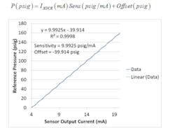
If you take your data and plot current (mA) on the x-axis and reference (actual) pressure on the y-axis and then do a least squares fit of a first degree polynomial to the data (fit a straight line through it), then the slope is your sensitivity in units of psig/mA and your offset is the intercept in psig (Figure 5). This means that, when you make a test measurement:

Figure 5: This is an exemplary calibration plot of a nominally 0-160 psig pressure transducer with a 4-20 mA output.

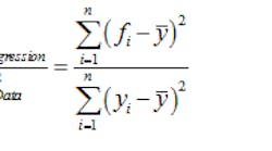
Your coefficient of determination, or R², should be noted, as well. This is a measure of how well you were able to fit the line to the calibration data, and is calculated as:

where y_i is an individual data point, f_i is the calculated fit for an individual data point and y-bar is the average of all data points. If the fit goes through every data point, then:

and this is indicative of a perfect linear fit. We want R² = 1, but in the real world, which isn’t perfect, they can’t be equal. Also, looking at the variance of a straight line, which we can say is nominal, as the sensitivity will be nominally the same for all sensors of the same type, we can say that the upper term just is what it is. So we want to minimize the lower term, or data variance, which means we want the variance of our data to be that of our straight line. Hence, R² is one measure of how well the data’s variance can be attributed to the fact that it should be a straight line, and we want all of its variance to be attributed to this fact.

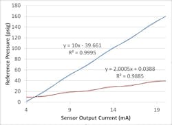
However, coming up with one gold standard R² value above which is good for all data isn’t possible. R² can be misleading. When each function has the same fit error (using the same error generation function for both curves) but the variance of the red line (shallower slope) is smaller, it results in a lower R² value. This demonstrates why you will need to do some investigating to set a meaningful minimum R² value (Figure 6).

Figure 6: These are two exemplary calibration curves with exactly the same magnitude of fit error.

Now, let’s establish limits on the sensitivity and offset and also consider checking each individual calibration data point.

Start with the sensor data sheet. If it’s nominally a 0-160 psig sensor with a 4-20 mA output, then your nominal sensitivity and offset values will be 10 psig/mA and -40 psig, respectively. This means that you should be generating numbers close to these if you perform good calibrations.

The next part is optional, but it’s suggested as part of a thorough repeatability and reproducibility study.

Run calibrations on many of these sensors, if available, and run each sensor through several calibrations, recording the calculated sensitivities and offsets. This will give you the expected sensitivity and offset values and variances within the entire population of sensors, as well as how these values behave for an individual sensor—its natural randomness.

Now plot the sensitivities vs. calibration number for all sensors, or multiple plots with subsets, if that’s easier to visualize. Do the sensitivities of any one sensor jump around more than the others? If you calibrated enough sensors, you may have a dud or two in there to do this with. What’s different about the raw data (pressure vs. current) curves? Is there anything way off in the sensitivities, offsets or R² values? If it looks not so linear, if you fit a quadratic or cubic to all calibration curves, how do the x³ and x² coefficients of the suspect sensors compare to the others? They should be higher, and the good sensors should have values close to zero for both of these coefficients. If so, this is something you can use to flag a potentially bad calibration and/or sensor.

Are your sensors being routinely calibrated? Are your skids kept in-house and you calibrate/check the instrumentation on them every so many days, weeks or months? If so, this takes a lot of guesswork out of the analysis. Running several or more sensors through a calibration and looking at their sensitivities and offsets will give you an idea of their expected normal values of that sensor type, but, in tracking historical data, you can expect a far smaller variance in those values. In the previous pressure transducer example, you may see 90% of all pressure transducers you calibrate will have sensitivities at some mean +/-0.8 psig/mA, but 90% of all transducers never left a range of +/-0.01 psig/mA over the course of so many years. Hence, if you detect a sharp deviation from a sensor’s own historical data, you can flag it for review, strictly by the numbers alone. Furthermore, although an acceptable transducer may have a sensitivity that falls within, say, 5% of the nominal sensitivity, if one specific transducer jumps from the upper end to the lower end of that range, or vice versa, then it should be flagged for review.

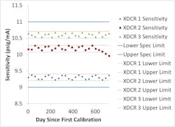
Figure 7: This is an exemplary SPC plot of historical sensitivities for three pressure transducers, nominally 4-20 mA output over a range of 0-160 psig, with a device limits of ±10% and specified hysteresis of ±1%.

A good starting point for these numbers is their repeatability or hysteresis ratings (%) on their data sheets, as that can be interpreted as there being something wrong with a sensor that is outside of these tolerances.

An individual sensor’s data can be used to establish its own unique limits, which are more restrictive than the specified accuracy tolerance of the device (Figure 7). Notice how the sensitivity of Transducer 2 is outside of its own hysteresis limits—not “acting like its usual self”—but well within the range of expected values for transducers. This is certainly not definitive proof that the transducer is faulty, but it’s strong evidence suggesting that it could be, so it should be flagged for review.

Establishing limits on each individual data point sets a considerably higher standard for a passing calibration, as just a single point out of potentially hundreds can cause a failed calibration. However, if it’s caused by something that’s not indicative of a sensor issue, such as a loose electrical connection between the DUC and DAQ, dumb luck, natural randomness or a fluke, then repeating the calibration procedure and producing a passing result should be no problem. The faulty sensors are the ones likely to repeatedly fail a calibration, so I highly recommend this approach with a three-strikes policy: three consecutive failed calibration attempts flags a DUC for removal.

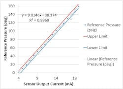
I almost can’t stress data visualization enough, especially in the infancy of this process. Numbers can be misleading. In Figure 8, the measured pressure oscillates in a range of 10 psig—a range that, relative to most sensor performance, is wide enough to land a 747—but its R² value, 0.9969, may appear to be very close to 1, and give the impression that the data is very good. Visualizing the data will yield meaningful interpretations of the numbers: Do you know what you’d call a bad R² value? What if all sensors are performing within spec, but one has a sharp relative deviation, still within the hysteresis limits? The deviation from “the usual” likely wouldn’t have stuck out in a table, as it would still be less than the spec limit, but would be more likely to stick out in a graph. Visualizing data will help you to establish a picture of what “the usual” should look like, so that you can be mindful of deviations.

Figure 8: If the outlier (third from last point) can be attributed to natural randomness, then repeating the calibration and producing a plot without that glitch shouldn’t be a problem. If it is, it’s more likely to be a bad sensor.

If you investigate a deviation that just doesn’t look quite right and then find that the sensor is malfunctioning, you may later ask: Why didn’t the calibration R²/sensitivity/offset/raw data fail some sort of limit comparison? You may determine that the limit was set too liberally, allowing bad sensor calibrations to pass. Conversely, if you are seemingly flagging sensors for review left and right, your limits may be too tight. Being able to verify that its raw calibration curves and historically calculated sensitivities and offsets appear to be normal, and there is nothing abnormal about results from parts tested with that sensor, will give indications that the limits for the parameter that sensors are being flagged for are too tight.

Natural randomness is expected in calibration data and calculated sensitivities and offsets, but all expected to be a relatively small range of variation, meaning that a considerable variation in any of these predicted behaviors is indicative of a potentially faulty sensor. Conversely, a sensor calibration that is within all limits set for the discussed metrics has a very low probability that either the calibration was performed incorrectly or that the sensor is malfunctioning (your escape probability is very low). Visualizing historical calibration data, especially in the infancy of this calibration process, is highly valuable in determining optimum statistical-process-control (SPC) limits in development and serves as an aid for troubleshooting for the life of the test systems.

Conclusion

These aren’t the only requirements of a good calibration, but in my line of work I’ve seen calibration processes done many different ways at many different places, and this is my recollection of what I’ve seen work out best, as well as areas to look into when it comes to designing and validating calibration procedures for your DUCs and reference units.

Building automated of semi-automated calibration and SPC capabilities into software is well worth the repeatability and reproducibility it buys you, and it is by far the best way to enforce the traceability required in a medical device environment. Development costs can be justified by comparing them to the cost of extra labor spent troubleshooting test systems or, depending on the application, escapes and subsequent product recalls. Both the calibration and SPC software capabilities can be built in such a way that doesn’t require re-validation of existing code.

Homepage image courtesy of renjith krishnan at FreeDigitalPhotos.net